A fully connected classification network example

In this section there is a brief example of solving a classification problem with a fully connected neural network with one hidden layer. This means that the network is formed of an input layer, a hidden layer, and an output layer, with the output of one layer flowing into the next with every neuron of one layer connected to every neuron of the next layer, hence fully connected. The main difference between a classification and regression network is the use of a softmax activation function to compress the output of the final layer into a 0 to 1 range which can be used for prediction of classes, multiple classes would typically mean an output vector with probabilities for each class in each element.

Although this is a basic neural network, it will highlight the main components of creating and training a typical neural network:

1. Data input and test/train split creation
2. Pre-processing
3. Network architecture
4. A loss function
5. A optimization routine
6. Training
7. Displaying training results

First, import the necessary libraries

import numpy as np
import matplotlib.pyplot as plt

# Make NumPy printouts easier to read.
np.set_printoptions(precision=3, suppress=True)

import tensorflow as tf
from tensorflow import keras
from tensorflow.keras import layers
import tensorflow_datasets as tfds 

from sklearn.model_selection import train_test_split

1. Data input and test/train split creation

We'll load a toy dataset from tensorflow-datasets (a package which must be installed). We are going to use the Iris dataset which has 50 examples with 4 features for each of 3 classes of irises. More information can be found here. We'll also use the train_test_split function from sci-kit learn to make our train and test datasets.

# load the dataset from tensorflow datasets
ds = tfds.load('iris', split='train', as_supervised=True)

# !NOTE - the .fit method expects batches so if we don't batch then we'll run into dimension mismatch issues when trying to train
# We'll split the dataset into training and test data and then further split the training dataset into a train and validation dataset
train, test = tf.keras.utils.split_dataset(ds, left_size=0.9, seed=0)
train, val = tf.keras.utils.split_dataset(train, left_size=0.9, seed=0)
train = train.batch(45)
val = val.batch(8)
test = test.batch(8)

Pre-processing

Typically the data that we work with isn't quite perfect for use in our models. We usually apply transformations to the data in order to make it optimal for our modelling purposes. The transformations could take the form of:

1. Formatting
2. Encoding
3. Normalization
4. Feature engineering
5. Feature selection

This is a non-exhaustive list and we'll go through pre-processing in more detail in another notebook. For now, we'll just apply a normalization layer to our input features. Because we have a batched input this makes simple normalization slightly more difficult. For example, do we normalize over the entire dataset or individual batches? In many real world scenarios we won't have the full dataset loaded into memory to be able to calculate the whole training dataset mean and standard deviation used for normalization. Here, we'll use BatchNormalization on the input to the model. Given our data is so small, it would be better to load all the data into memory and normalize over the entire dataset, but we'll stick with the BatchNormalization approach for educational purposes. We will define the BatchNormalization as a layer when we build our model in Keras.

Network Architecture

Training a model with tf.keras typically starts by defining the model architecture. Here, we use a tf.keras.Sequential model, which represents a sequence of steps. We will be training a simple classification model to attempt to map between the input features and the target labels using fully connected layers (tf.keras.layers.Dense) with a ReLU activation function for the single hidden layer and a softmax activation function for the output layer. The number of inputs can either be set by the input_shape argument, or automatically when the model is run for the first time. Note, however, that without defining the input shape then we can't show a summary of the model using the summary method (as the input shape will still be unknown until we run it on data).

linear_model = tf.keras.Sequential([
    layers.BatchNormalization(),
    layers.Dense(units=5, input_shape=[4,], activation='relu'),
    layers.Dense(units=3, activation='sigmoid')
])

Loss function and optimization

Once we have built the architecture of the model, we configure the training procedure using the Keras Model.compile method. The most important arguments to compile are the loss and the optimizer, since these define what will be optimized (mean_absolute_error in this example) and how (using the tf.keras.optimizers.Adam). We also specify a hyper-parameter here for the optimizer in terms of the learning rate. This, for the time being is a choice that has been made using prior knowledge of what works well. Hyper-parameter optimization is a topic in it's own right and will be covered in a different notebook. Note that we use the SparseCategoricalCrossentropy as our labels as provided as integers and not one-hot encoded. Further more, as per the documentation: "There should be # classes floating point values per feature for y_pred and a single floating point value per feature for y_true." Which is why we have a final output layer with # of classes units.

linear_model.compile(
    optimizer=tf.keras.optimizers.Adam(learning_rate=0.25),
    loss=tf.keras.losses.SparseCategoricalCrossentropy(),
    metrics=['accuracy'])

Training

Once the model has been built and the training routine defined in the compile method then we can execute training using the fit method of our Keras model. Another hyper-parameter of note here is the number of epochs. This is set manually here, but can also be optimized using early stopping criteria. We store the output of the training in the history variable to be able to store, analyze, and visualize metrics about the model training.

history = linear_model.fit(
    train,
    epochs=200,
    verbose=0,
    validation_data = val
    )

We can now evaluate our trained model on the test dataset. The returned values from the evaluate method on the model are the loss value and metric values for the model in test mode link to documentation.

evaluation = linear_model.evaluate(test)
for name, metric in zip(linear_model.metrics_names, evaluation):
    print('test ' + name + ': ' + str(metric))
    

test loss: 0.02136881649494171
test accuracy: 1.0

visualization of training metrics

Now that the training has finished we can visualize the model's training progress using the metrics stored in the history object:

def plot_loss(history):
    plt.plot(history.history['loss'], label='loss')
    plt.plot(history.history['val_loss'], label='val_loss')
    plt.plot(history.history['accuracy'], label='accuracy')
    plt.xlabel('Epoch')
    plt.ylabel('Error')
    plt.legend()
    plt.grid(True)
    plt.ylim([0,2])

plot_loss(history)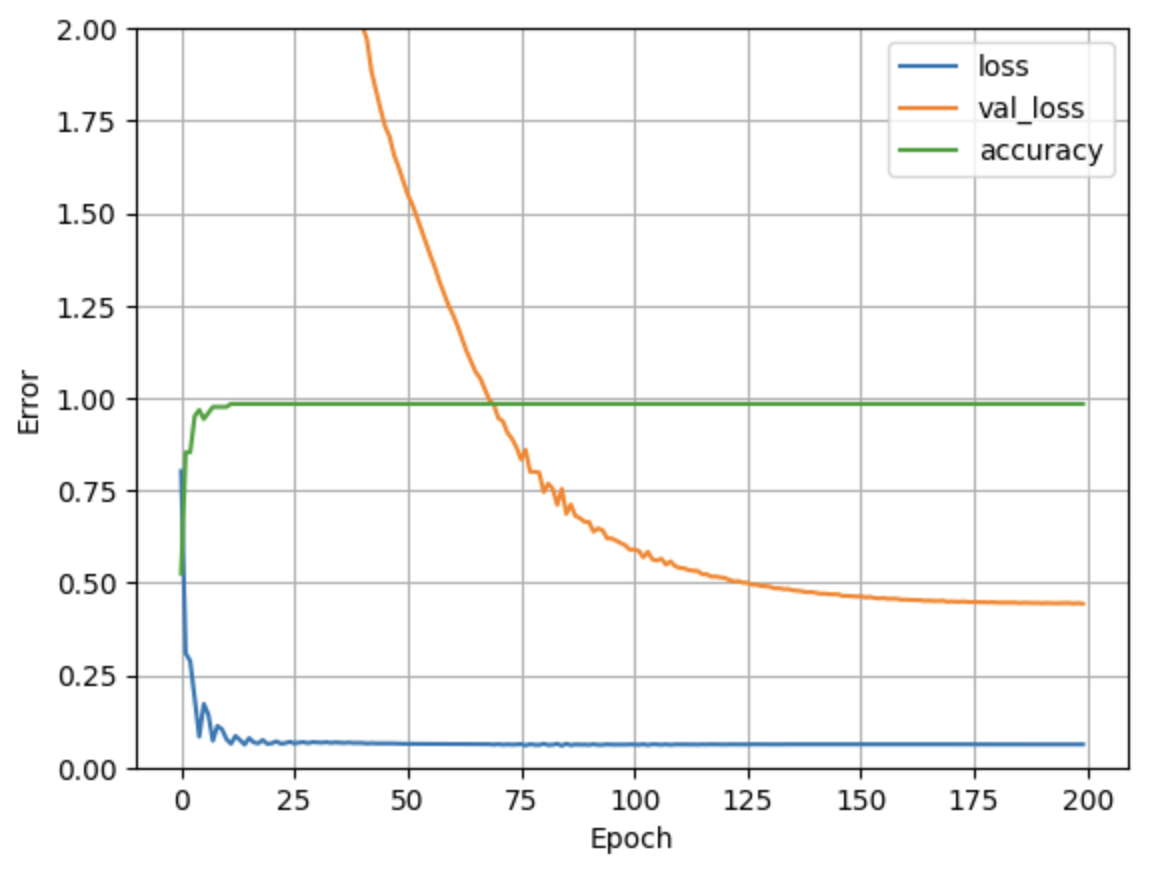

Now that we have a trained model we make predictions by passing in our new data.

linear_model.predict([[6.4,2.8,5.6, 2.2], [5.4, 3.4,1.7, 0.2], [5.9, 3.,  4.2, 1.5]])

array([[0.   , 0.   , 0.465],
    [1.   , 1.   , 0.039],
    [0.   , 0.994, 0.135]], dtype=float32)

Summary

In this topic we've gone through a simple example of building a fully connected neural classification network. Next, have a look at the maths behind the neural network we've built in this topic:

This work is licensed under a Creative Commons Attribution-NonCommercial-ShareAlike 4.0 International License.