Non-linear least squeares inversion

An example of why non-linear inversion is needed

We have seen in the previous sections how to perform linear inversion and even how to linearize a problem to solve it in the framework that we set up for the linear case. But in some cases we won't be able to solve our problem in a linear manner. We'll highlight this by introducing a real world problem that can't be linearized.

The problem we will look at involves infra-red spectrometry data from massive young stellar objects (MYSOs). These objects are young stars that are still forming and gaining mass from accretion disks that deposit material on the star. As part of this process, jets of material are expelled at the poles of the MYSOs. By looking at absorption spectra from these MYSOs of certain transition of hydrogen with known frequencies then we can approximate how much mass is being ejected from these poles and gain a slight understanding of whether the pole is orientated towards or away from us. The width and depth of the absorption spectra give an understanding of the mass loss rate as a larger cone will have a wider range of incidence angles with the Earth and hence a wider spectrum (as some is blue shifted and some is red-shifted due to the velocity of material relative to the Earth) and a deeper absorption line is a indicative of a higher density of material. So what do these spectra look like?

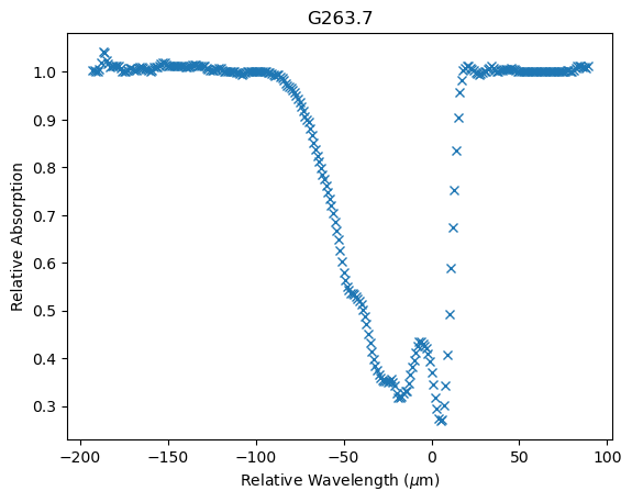
Given this it makes sense to try to fit Gaussian curves to the absorption spectra to give an estimate of the width (the standard deviation of the Gaussian) and the depth (the amplitude of the Gaussian). The centre point of the Gaussian can also tell us whether the absorption line as a whole is red- or blue-shifted to give us some information about the speed of the MYSO relative to the Earth. So what would be the form of the Gaussian we want to fit? First note that the absorption spectra could be modelled not by multiple Gaussian curves but by "negative" Gaussian curves with a baseline at 1 (i.e. just add 1 to the distribution). It is also apparent that the absorption spectra could have multiple different components which can be attributed to distinct ejection events or periods, but we'll only focus on fitting a single Gaussian here. The form of the model representing the absorption spectra (or at least one Gaussian component of it) is:

$$ \LARGE{y = 1 - A e^{\frac{-(x-\bar{x})^{2}}{2\sigma^{2}}} }$$

where $in A $in is the amplitude of the Gaussian, $in \bar{x}$in is the location of the mean of the Gaussian, and $in\sigma$in is the standard deviation of the Gaussian.

It is clear to see that is isn't really possible to linearly separate the three model variables from the measurement axis, $in x$in, in this equation. So if we can't solve this problem as a linear least squares problem then one solution is to solve it as a non-linear least squares problem.

Non-linear least squares derivation

In linear least squares we have our problem in the form $in d = Gm $in because we can linearly separate the model variables from the physics encapsulated in the forward operator, $in G$in. However, in the case presented above we can't linearly separate the model variables so our problem can only be formulated as:

$$d=g(m)$$

Here the forward operator is a function of the model variables as we cannot separate the two. In non-linear least squares we don't attempt to directly solve this equation for the model variables, as was done before in the linear case. Instead, we start with a guess of the model parameters and attempt to update these model variables using the misfit between the calculated measurements using these model variables and the recorded values. How to define this update and traverse this misfit space is an entire subject in itself; optimization. This we will cover separately. Here we will derive and implement a basic optimization called gradient descent.

The equation we have been working with thus far can be reformatted into a cost function that we to minimize. We have already seen the cost function in action in the previous topics on linear least squares inversion, where we let the cost function be the L2-norm of the recorded values and the values that the model suggests they should be. In other words we can define our cost to be

$$C = ||d-g(m)||^{2}$$

Where $in C$in is the cost. The aim is to minimize this cost function, the lower the value of the cost function the better the fit. However, we aren't trying to update the initial guess model parameters directly for the best estimate model parameters in one go, we are looking for an incremental uplift on the current model parameter estimates, $in \delta m$in, such that the new model parameters lower the cost function metric. In this case the equation of the cost function becomes

$$C = ||d-g(m_{k} + \delta m_{k})||^{2}$$

And we are trying to optimize for the model update, $in \delta m$in. To do this though we will need to expand the data kernel, $in G$in, such that we have a function that is solely dependent upon the model update, $in \delta m$in. We can do this by performing a Taylor series expansion on the cost function around the current model estimate, $in m_{k}$in.

$$ g(m_{k} + \Delta m) = g(m_{k}) + \frac{\partial g}{\partial m}\big\rvert_{m_{k}} \Delta m + \frac{1}{2}\Delta m^{T} \frac{\partial^{2} g}{\partial m^{2}}\big\rvert_{m_{k}} \Delta m $$

If we assume that the model update is small then any quadratic terms in the change in model parameters (or higher) can be regarded as negligible and ignored. The partial derivative of the forward operator with respect to the model parameters evaluated at the current model parameter estimates, $in \frac{\partial g}{\partial m}\big\rvert_{m_{0}}$in, is referred to as the Jacobian and usually given the symbol $in J$in. Along with ignoring factors in the expansion which are at least quadratic in the model update leads to

$$ J = \frac{\partial g}{\partial m}\big\rvert_{m_{k}} $$ $$d = g(m_{k}) +J\Delta m $$

Which means the cost function to optimize is

$$c = \begin{Vmatrix} g(m_{k}) - Y + J\Delta m \end{Vmatrix}^{2} $$

From here we can take the usual approach of taking he derivative with respect to the parameter to optimize and set the result to 0, re-arrange and solve for the parameter to optimize, which in this case is the model update.

$$\frac{\partial C}{\partial m} = 2J^{T}( g(m_{k}) - Y + J\Delta m) = 0$$ $$J^{T} (g(m_{k}) - Y) + J^{T} J\Delta m = 0$$ $$J^{T} J\Delta m = -J^{T} (g(m_{k}) - Y) $$ $$\Delta m_{k} = -(J^{T} J)^{-1} J^{T} (g(m_{k}) - Y) $$ $$m_{k+1} = m_{k} - (J^{T} J)^{-1} J^{T} r $$

What is listed here is for the first iteration only due to the $in m_{0}$in term but it is trivial to generalize this to any iteration

$$m_{k+1} = m_{k} - (J_{k}^{T} J_{k})^{-1} J_{k}^{T} r_{k} $$

Solving our Gaussian fitting problem with non-linear least squares inversion

Now we have a framework for solving problems in non-linear least squares inversion we'll use it to solve our original problem of fitting Gaussian curves to infrared spectrometry data. The function we want to fit is

$$ \LARGE{y = 1 - A e^{\frac{-(x-\bar{x})^{2}}{2\sigma^{2}}} }$$

We now have to form the Jacobian matrix, $in J$in, via taking the partial derivative of the equation for the target variable with respect to each model parameter.

$$\LARGE{\frac{\partial y}{\partial A} = -e^{\frac{-(x-\bar{x})^{2}}{2\sigma^{2}}}} $$

$$\LARGE{\frac{\partial y}{\partial \bar{x}} = -A\frac{(x-\bar{x})}{\sigma^{2}}e^{\frac{-(x-\bar{x})^{2}}{2\sigma^{2}}}} $$

$$\LARGE{\frac{\partial y}{\partial \sigma} = -A\frac{(x-\bar{x})^{2}}{\sigma^{3}}e^{\frac{-(x-\bar{x})^{2}}{2\sigma^{2}}}} $$

Now that we have our equation for the Jacobian entries for each model parameter then all that is left to do is read in the data, generate some initial guess of the model parameters and iterate around this loop until the misfit doesn't seem to be decreasing. Note that there is lot to unpack here in terms of when to stop iterations, where put your initial guess etc. and these issues can have very large impacts on the results you obtain. The optimization algorithm may not (probably won't) find a optimum result if the initial guess is too far from the best fit model parameters. This is because, among other things, there could be little misfit surface gradient to guide your optimization algorithm, and the further you get away from the global minimum (if there is one) then the more likely you optimization algorithm is to fall into a local and not global minimum.

Solving our Gaussian fitting problem with non-linear least squares inversion - python implementation

First, as usual, let us read in some libraries and define the functions that will be doing the inversion, based on the equations we derived above

import json
import numpy as np
import matplotlib.pyplot as plt

def plotting(x, y, m, xlabel, ylabel, polynomial_degree):
    plt.figure()
    plt.plot(x,y,'x')
    plt.xlabel(xlabel)
    plt.ylabel(ylabel)
    plt.title(f'{ylabel} Vs {xlabel}')
    xfine = np.linspace(np.min(x), np.max(x), 10*len(x))
    G = makeG(xfine, polynomial_degree)
    yfine = np.dot(G,m)
    plt.plot(xfine,yfine,'r--')

def makeG(x, m):
    G = np.zeros((len(x), 3))
    exponent = np.exp(-np.power((x - m[1]),2)/(2*np.power(m[2],2)))
    G[:,0] = -exponent
    G[:,1] = -m[0] * (x - m[1]) * exponent / np.power(m[2],2)
    G[:,2] = -m[0] * np.power((x - m[1]),2) * exponent /(np.power(m[2],3))
    return G

def forwardModel(x, m):
    y_hat = 1 - m[0] * np.exp(-np.power((x - m[1]),2)/(2*np.power(m[2],2)))
    return y_hat

def linearInversion(x, y, m, lam):
    G = makeG(x, m)
    Gt = G.T
    GtG = np.dot(Gt, G)
    GtGinv = np.linalg.inv(GtG)
    m = np.dot(np.dot(GtGinv, Gt), y)
    return m

Note that not much has changed in the helper functions we have defined to carry out our inversion compared to the linear least squares case. The only structural difference is that we have now have a "forwardModel" function to generate the expected output data given the current model parameters that will be used to compared with the recorded data.

The next thing we do is load the infrared spectrometry data from the JSON file, which can be accomplished via the inbuilt JSON package, and normalize the data by it's median, making sure that the baseline is set to 1.

file = 'G263.7.json'
with open(file, 'r') as f:
    js = json.load(f)

for key in js:
    js[key]['y'] = js[key]['y'] - np.median(js[key]['y']) + 1.0

We know need to figure out how to provide a good initial estimate of the model parameters. This will depend on the individual problem you are solving adn the domain expertise that could be utilized (or even required). In this problem we know we are trying to fit Gaussian curves and need to generate an initial guess for the amplitude, location, and width of the Gaussian. We can get a good estimate of the initial amplitude and location by simply looking for the minimum amplitude (value) in the array of data, minimum because it is an inverted Gaussian. The width we could estimate via some means but for this toy example we can just look at the data (which is a valid method for smaller datasets) and use an initial guess of 5$in \mu m$in.

index = np.argmin(y)
m = [1.0 - y[index], x[index], 5.0]

Now that we have the the helper functions defined and an initial guess all that is left is to loop through updating those initial model parameters with the update given by the non-linear inversion.

Nepochs = 10
norm_history = 0
for iteration in range(Nepochs):
    y_hat = forwardModel(x, m)
    r = y_hat - y
    dm = linearInversion(x, r, m)
    m -= dm
    plt.plot(x,y)
    plt.plot(x,y_hat);plt.show()
    print(f'data norm: {np.linalg.norm(r,2)} model norm: {np.linalg.norm(dm)}')
    if np.abs(np.linalg.norm(r,2) - norm_history) < 0.01:
        break
    else:
        norm_history = np.linalg.norm(r,2)

You may notice that we added an if statement into the loop to compare the current loss with the loss generated from the previous model. If the loss is below a given threshold, hard-coded to 0.01 here, then the iterations terminate. This is known as an early stopping criteria and the are widely used to save compute and time resources. After a while, the model becomes as good as it can be, it gets stuck in a minimum of the loss surface, hopefully the global minimum, but iterating further won't change teh results of the model or the parameters and is wasted energy.

Interestingly, our initial guess of the best model parameters for fitting a single Gaussian were off by quite a bit. This is because the method we used to estimate the initial model parameters used the largest amplitude. However, if one wants to reduce the cost function as much as possible then it is more important to account for the Gaussian that has the largest contribution to cost function, which in this case is one that is lower in amplitude but much wider, giving it a great area within our data range than the Gaussian corresponding to our initial guess. This is a cautionary tail, your initial guess may be correct, but it may not be "best" answer.

The aim of these first few topics in the inverse theory series has been to get you up to speed as quickly as possible to implement solutions yourself. Our focus has been on implementation and not mathematical rigour. However, in doing so we have overlooked a few key points that need to addressed before diving into the next addition to our set of tools to solve inverse theory problems. In the next topic we'll cover some more fundamental information and learn how to implement, and estimate errors from solution to our inversion problems.

Fundamentals and Covariance Matrices