Digital Series Analysis basics

Basic characteristics of digital signals

Digital signals are measurements of some real world phenomenon but unlike those phenomena they are not continuous, they are snapshots taken at specific time intervals. It is important to know some of the basic characteristics of these digital signals to avoid some common pitfalls when further interpreting or analysing them. We'll start by looking at a 1-dimensional time series and some of the basic attributes that they have but the theory can be extended to any number of dimensions. We'll see later an example of a 2D digital series. One other thing to note is that unless stated otherwise we will assume that the series is regularly sampled such that each data point is measured at a fixed distance (in whatever measurement untis are appropriate) from the next sample point. We will touch on irregularly sampled data in a later notebook.

A digital signal itself is remarkably simple in how many attributes it has, which is essentially 1, the number of samples. Any transformation we care to do with the signal can be applied without knowing any information other than how many samples are int he signal. All other information can be seen as "meta-data", which is information about the signal but not an inherent characteristic of the signal. This may change how we label certain axes and the units used but the underlying algorithms should be agnostic of the units. Only in advanced modelling where, for instance, the time of the recorded event is used within the algorithm to correlate to other, external, datasets will this meta-data make an appreciable difference in how the algorithms and transformations we will investigate work.

Having said all that, the meta-data that should accompany a digital series is extremely important as it is the context around the digital series. Without context, any analysis and interpretation of the signal could not any meaningful conclusions, making it of limited use in a real world setting. So, let's now look at some common, and important, meta-data that should accompany any digital series. I'll also list some common synonyms of these terms, but please bear in mind that the terminology varies not only between different industries/fields but also within them too.

• Sampling interval/recording interval/sample interval - This is the distance between two sample points in the units used to record the data. For instance if we recorded the temperature every second then the subsequent time series would have a sampling interval of 1 second.
• Sampling rate/sampling frequency/recording frequency - This is simply the inverse of the sampling interval, which for the above example would mean that the sampling rate is 1 per second. Note that instead of "per second" you might see the sampling rate given in units of Hertz (Hz). Hertz is a measure of cycles per second, such that 10Hz is 10 cycles per second.
• Total signal length - Usually this can be calculated from knowing the number of samples and the sampling interval but in the uncommon situation when the only the length of signal and number of samples is known then the sampling interval can be calculated from this number.

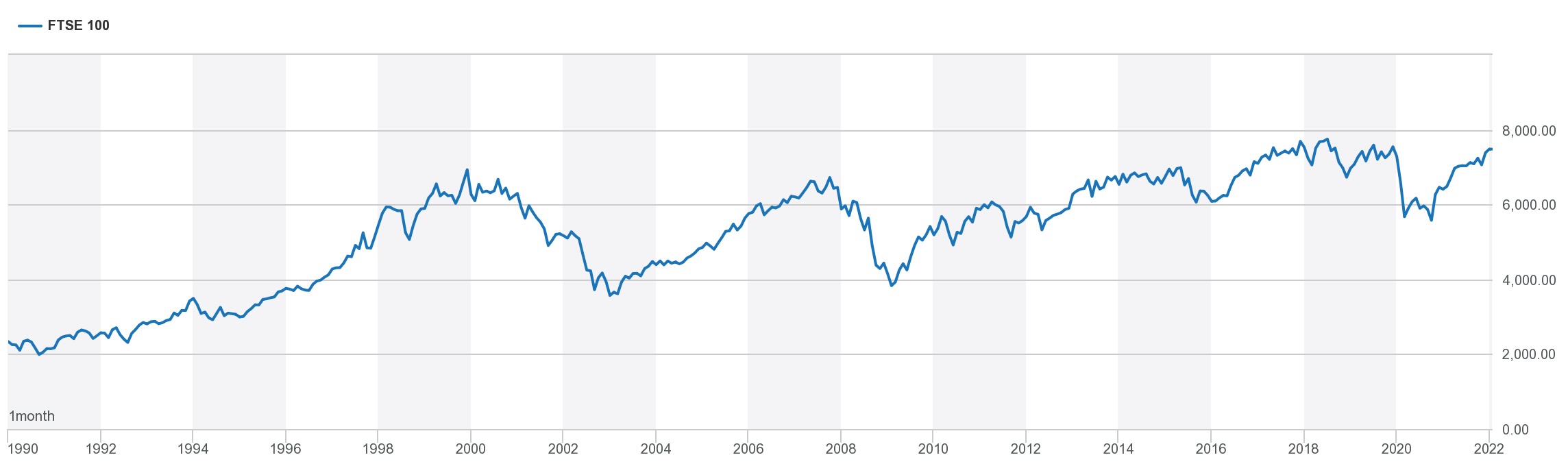
Other meta-data which can be vitally important but depends on your particular use case and can include the time and/or location that the data was recorded, how it was recorded, what instruments were used, or the distance to any source of energy used in active recording, this is a non-exhaustive list but shows how much information can be incorporated beyond just the signal itself. External data that is not directly associated with the recorded digital series can also be incorporated if it provides insight into the data at hand. For instance; looking at the historic trend of a stock market in the image below it would be important to note that there were financial crises in the late 1990's and late 2000's brought about by different factors. Without this context, and looking at the series from 1990 to 2012, one could draw the conclusion that a stock market crash would be expected once every decade as a natural cycle, when we know this isn't the case.

The importance of the basic characteristics of digital series

The two main pieces of meta-data we have considered thus far are the number of samples and the sampling interval (or inversely the sampling rate) or the the total length of the series in measurement units (as we can freely convert between the two). Now let's look at why they are so important.

As we have previously seen in the case of the stock market example, we might want to understand common cycles within our series of data. These cycles will have a particular frequency such as once every 10 years, or 5 times per second. Hertz (Hz) is commonly used to denote frequency as is the number of cycles per second (1/s). Frequencies can be extremely low or extremely high; for instance winter comes once per year (a frequency of 3.17x10^-8Hz!) where as the middle C sound in music is approximately 262Hz and the radio that we listen to is carried on waves between 87Mhz and 108Mhz (8.7x10 ⁷Hz to 1.08x10 ⁸Hz) in the UK. That's a big range, and by no means the limits!

Given this huge range of frequencies, how should we set up our recording equipment to be able to record these signals? It seems intuitive that if we want to measure something that varies on the scale of a year that we should record for longer than a second and if we want to record something that is changing rapidly then we need to take measurements very quickly too.

We will formalise this mathematically but first let's look at a quick example. Below is a series of code cells to run that will show you how altering the recording interval for a simple sine wave alters the measured signal appearance, sometimes to dramatic affect.

# let's import some useful libraries
import numpy as np
import plotly.offline as pyo
import plotly.graph_objs as go
import matplotlib.pyplot as plt
pyo.init_notebook_mode()
plt.rcParams['figure.figsize'] = [12, 8]
# %matplotlib inline

def Plotting(ys, xs, labels, slider_labels, title=None,slider_prefix=None, slider_suffix=None, first_visible=True, mode='lines+markers', dash=None):
    '''
    Helper function for producing plots given a signal and some sampling intervals
    '''
    data = [dict(
            mode = mode,
            visible = False,
            line = dict(color='#00CED1', width=4, dash=dash),
            marker = dict(symbol='star', size=12),
            name = labels[step],
            x = xs[step],
            y = ys[step]) for step in range(len(xs))]
    data[1]['visible'] = True
    if first_visible:
        data[0]['visible'] = True
        data[0]['mode'] = 'lines'
        data[0]['line'] = dict(color='#000000', width=6)

    steps = []
    for i in range(1,len(data)):
        step = dict(
            method = 'restyle',
            args = ['visible', [False] * len(data)],
            label = slider_labels[i]
        )
        step['args'][1][i] = True # Toggle i'th trace to "visible"
        if first_visible:
            step['args'][1][0] = True
        steps.append(step)

    sliders = [dict(
        active = 0,
        currentvalue = {"prefix": slider_prefix, "suffix":slider_suffix},
        pad = {"t": 50},
        steps = steps
    )]

    layout = dict(sliders=sliders)
    fig = dict(data=data, layout=layout)

    print(fig)
    
    pyo.iplot(fig, filename=title)

# set up time axis
Nsamp = 2000 # number of samples
dt = 0.01 # sample interval
L = (Nsamp - 1)*dt # Time length of signal
t = np.linspace(0,L,Nsamp) # vector of time instants

# create a sine wave
f = 1 # best to keep this the same for the comparisons
sig = np.sin(2 * np.pi * f * t) 
sampling_intervals = np.arange(5,400,80) # these are the sampling intervals we will use measured in samples, not time!
ts, sigs, labels= ([],[],[])
for step in sampling_intervals:
    ts.append(t[::step])
    sigs.append(sig[::step])
    labels.append('Measured Signal')
labels[0] = 'Sine wave'

Plotting(sigs, ts, labels, slider_labels=(sampling_intervals*dt).astype(str), title='Sine Wave Slider', slider_prefix="Sampling interval: ", slider_suffix="ms", dash='longdash')

Note that when the samping interval is an integer multiple of the inverse of the frequency we are trying to observe (the sine wave in this case) then the same point is measured on each cycle and a flat signal is measured, showing no variation at all. Although in the above example a flat response was also given for a sampling interval equal to half the inverse of the frequency of the sine wave this is a peculiarity of the data and as can be seen from the below example, which is just phase shifted slightly. We can see that there is identifible information at a sampling interval of half the inverse of the frequency we are trying to observe.

# create a sine wave with a phase shift
sig = np.sin(2 * np.pi * f * t + 0.5) 
        
sigs = [sig[::step] for step in sampling_intervals]
        
Plotting(sigs, ts, labels, slider_labels=(sampling_intervals*dt).astype(str), title='Sine Wave Slider', slider_prefix="Sampling interval: ", slider_suffix="ms")

If you look at the sampling intervals between half the inverse of the sine frequency and the inverse of the sine frequency then you'll notice that the measured signal looks to be progressively lower frequency until we hit the constant (essentially "zero-frequency") signal. This is because we are taking less than 2 measurements per cycle of the wave which results in successive measurements being further along the next cycle than the previous measurement, essentially stretching the appearance of the measured signal, making it appear to be of a lower frequency. This becomes more pronounced the further apart the samples become (the higher the sampling interval, or conversely the lower the sampling rate) until we only record 1 sample per cycle, which for a sine wave becomes the same value and thus a flat signal.

This is a fundamental and important aspect of digital series; the Nyquist frequency. Check it out in the next page:

The Nyquist Frequency