Fourier Transforms - looking at the frequencies

All you need is sines

We have introduced frequencies and even tried to assess qualitatively the appearance of a signal in terms of "higher" and "lower" frequencies. But how can we quantitatively assess the frequencies of a signal? If we could fit an analytic signal, or series of them, to a form a spike then we could fit any digital signal as a digital signal is, in essence, a series of spikes of varying amplitude at distinct measurement points. It turns out that a series of sine (or cosine) waves with various amplitude, frequency, and phase can be fit together to from a spike. Specifically, one could sum cosine waves of zero phase, constant amplitude, and varying frequencies to generate a spike at t=0. Then all that is required to phase shift the component cosines to move the spike in time.

short_time = np.linspace(-1.5,1.5,101) # generate symmetric time axis around 0
FNyq = 1/(2*(short_time[1] - short_time[0])) # get the Nyquist frequency
freq_interval = 0.01 # define frequency interval to use
freqs = np.arange(freq_interval, FNyq+freq_interval, freq_interval) # generate a list of frequencies to make sine waves for, up to Nyquist
evr = 50

# set up array of signals and legends
combined_signal = np.cos(2 * np.pi * freqs[0] * short_time)
ys_cos=[combined_signal.copy()]
leg_cos = ['Frequency: '+str(freqs[0])]

# loop over frequencies
for i in range(1,len(freqs)):
    combined_signal += np.cos(2 * np.pi * freqs[i] * short_time)
    if i%evr==0: # only take a set number of intervals for plotting
        ys_cos.append(combined_signal/i)
        leg_cos.append(str(round(freqs[i],2)))

if i%evr!=0:
    ys_cos.append(combined_signal/i)
    leg_cos.append(str(round(freqs[i],2)))
        
# produce interactive plot
ts_cos = [short_time]*len(ys_cos)       
Plotting(ys_cos, ts_cos, leg_cos, slider_labels=leg_cos, title='Building a spike', slider_prefix="Sum of frequencies to: ", slider_suffix="Hz", first_visible=False, mode='lines')

inds = range(1,len(ys_cos),4)
for i in inds:
    plt.plot(ts_cos[i], ys_cos[i])
plt.legend(['Frequency: '+leg_cos[i] for i in inds])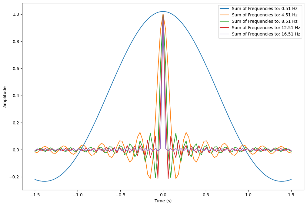

The above plot shows the sum of cosine waves of up to various frequencies. It turns out that a series of sine (or cosine) waves with various amplitude, frequency, and phase can be fit together to from a spike. Specifically, one could sum cosine waves of zero phase, constant amplitude, and varying frequencies to generate a spike at t=0. Then all that is required is to phase shift the component cosines to move the spike in time.

This means that any digital signal can be approximated by a series of cosines of varying amplitudes, frequencies, and phases. This is known as a Fourier series. The fitted amplitudes, frequencies, and phases can now be assessed to determine how strong each frequency is represented in the signal. For instance, one would expect a good fit for a cosine wave with a period of a year to data relating to average temperatures over time for the UK.

We can do this because, assuming there are no data points of infinite amplitude in our series, we only have finite discontinuities. This is one of the Dirichlet conditions that must be met to be able to represent a signal as a Fourier series. What would this look like mathematically?

$$ s(t) = \frac{a_{0}}{2} + \sum^{\infty}_{n=1}a_{n}\cos(2\pi n t/T+\theta_{n}) $$
Note that we have a coefficient out front of $\frac{a_{0}}{2}$ which accounts for the average of the signal. For instance if we wanted to fit a flat, non-zero response then $a_{0}$ would correspond to twice the average of the signal and all other coefficients would be zero. We can also write this equation in terms of sines and cosines without any phase term as sine and cosine form an orthogonal set:

$$ s(t) = \frac{a_{0}}{2} + \sum^{\infty}_{n=1}b_{n}\cos(2\pi n t/T) + c_{n}\sin(2\pi n t/T) $$
Where $ina_{n} = \sqrt{b_{n}^{2} + c_{n}^{2}}$in and $in\theta_{n} = \tan^{-1}\left(-\frac{c_{n}}{b_{n}}\right)$in.

This is a representation of a real valued series as a Fourier Series, however we can also extend this to complex valued signals as well by exchanging sines and cosines for a complex exponential:

$$ s(t) = \sum^{\infty}_{n=-\infty}a_{n}e^{2i\pi n t/T} $$
However, if we have infinitesimally small separations between the discrete frequencies then we can think of this series in terms of an integral: