A linear regression example with a fully connected network

In this section there is a brief example of solving a multi-feature linear regression problem by using a fully connected neural network with 1 layer, so there aren't any hidden layers. These kind of problems can also be solved using an inverse theory approach, and can be mathematically formulated to be the same assuming that we have linear activation functions on our neurons. See here for reference of how the problem of linear regression is solved from an inverse theory perspective: Simple mathematical tricks to force a linear problem

Although this is a basic neural network, it will highlight the main components of creating and training a typical neural network:

1. Data input and test/train split creation
2. Network architecture
3. A loss function
4. A optimization routine
5. Training
6. Displaying training results

First, import the necessary libraries

import numpy as np
import matplotlib.pyplot as plt

# Make NumPy printouts easier to read.
np.set_printoptions(precision=3, suppress=True)

import tensorflow as tf
from tensorflow import keras
from tensorflow.keras import layers

from sklearn import datasets
from sklearn.model_selection import train_test_split

1. Data input and test/train split creation

We'll load a toy dataset from sci-kit learn which has several toy datasets to use. We'll use the diabetes dataset which has 442 examples of 10 features with a separate target value. More information can be found here. We'll also use the train_test_split function from sci-kit learn to make our train and test datasets

# load the dataset
diabetes = datasets.load_diabetes()
features = diabetes['data']
target = diabetes['target']

# create the train/test split
train_feature, test_feature, train_target, test_target = train_test_split(
     features, target, test_size=0.05, random_state=42)

Here we have split the data into train and test datasets using the train_test_split function from sklearn.model_selection. We also use a fixed random state so that the training and test splits are consistent when we re-run the script

Network Architecture

Training a model with tf.keras typically starts by defining the model architecture. Here, we use a tf.keras.Sequential model, which represents a sequence of steps. We will be training a linear regression model to attempt to map between the input data and the target feature using a fully connected layer (tf.keras.layers.Dense) with a linear pass through activation function. If we don't specify an activation function in the creation of the fully connected layer (layers.Dense), then a linear ($ing(x)=x$in) activation is used. The number of inputs can either be set by the input_shape argument, or automatically when the model is run for the first time. Note, however, that without defining the input shape we can't show a summary of the model (as the input shape will still be unknown to the model until we run data through it).

linear_model = tf.keras.Sequential([
    layers.Dense(units=1, input_shape=[10]),
])

# call the summary method of the model to show a summary of the model that we have created
linear_model.summary()

            Model: "sequential_7"
_________________________________________________________________
 Layer (type)                Output Shape              Param #   
=================================================================
 dense_7 (Dense)             (None, 1)                 11        
                                                                 
=================================================================
Total params: 11
Trainable params: 11
Non-trainable params: 0
_________________________________________________________________
        

Loss function and optimization

Once we have built the model, we configure the training procedure using the Keras Model.compile method. The most important arguments to compile are the loss and the optimizer, since these define the loss function to be optimized which serves as a measure of accuracy for predicted outputs from the model (mean_absolute_error) and how we should optimize the model based on the outputs of this loss function (using the tf.keras.optimizers.Adam optimizer in this instance). We also specify a hyper-parameter here for the optimizer in terms of the learning rate, which we'll discuss in the optimizers topic. This, for the time being is a choice that has been made using prior knowledge of what works. Hyper-parameter optimization is topic in it's own right and will be covered in a different topic too.

linear_model.compile(
    optimizer=tf.keras.optimizers.Adam(learning_rate=0.2),
    loss='mean_absolute_error')

Training

Once the model has been built and the training routine defined in the compile method then we can execute training using the fit method of our Keras model. Another hyper-parameter of note here is the number of epochs. This is set manually here, but can also be optimized using early stopping criteria. We store the output of the training in the history variable to be able to store, analyze, and visualize metrics about the model training.

history = linear_model.fit(
    train_feature,
    train_target,
    epochs=200,
    # Suppress logging.
    verbose=0,
    # Calculate validation results on 25% of the training data.
    validation_split = 0.25)

visualization of training metrics

Now that the training has finished we can visualize the model's training progress using the metrics stored in the history object:

def plot_loss(history):
    plt.plot(history.history['loss'], label='loss')
    plt.plot(history.history['val_loss'], label='val_loss')
    plt.xlabel('Epoch')
    plt.ylabel('Error')
    plt.legend()
    plt.grid(True)

plot_loss(history)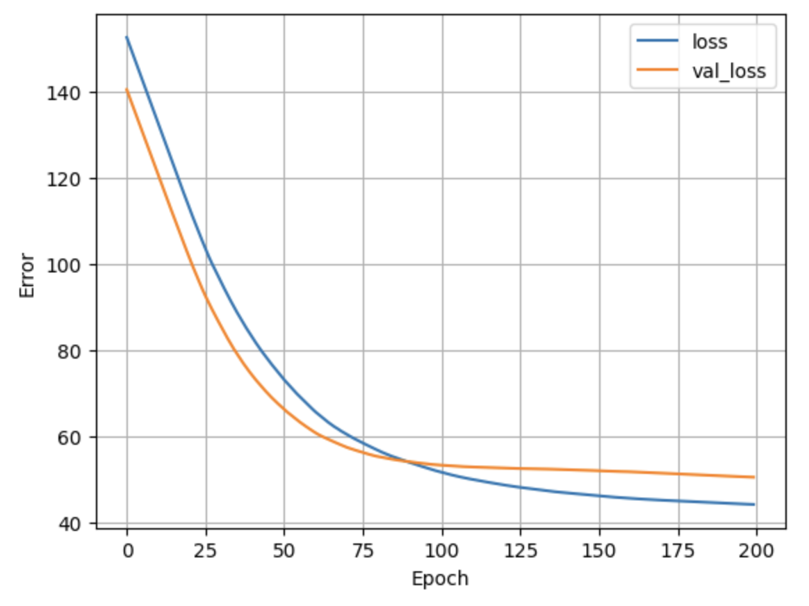

Now that we have a trained a model, let's see what the predictions look like on our test set. The easiest way to do this is to plot the predictions from the test features against the test labels. Ideally, they will be the same and we can visually inspect this by plotting them alongside a y=x line.

prediction = linear_model.predict(test_feature)
def plot_predictions(target, prediction, xlabel, ylabel):
    min_target = min(target)
    max_target = max(target)
    plt.figure()
    plt.plot(target, prediction, 'x', label='Data')
    plt.xlabel(xlabel)
    plt.ylabel(ylabel)
    plt.title(f'{ylabel} Vs {xlabel}')
    plt.plot([min_target, max_target],[min_target,max_target],'r--', label='x=y')
    plt.legend()

plot_predictions(test_target, prediction, '', '')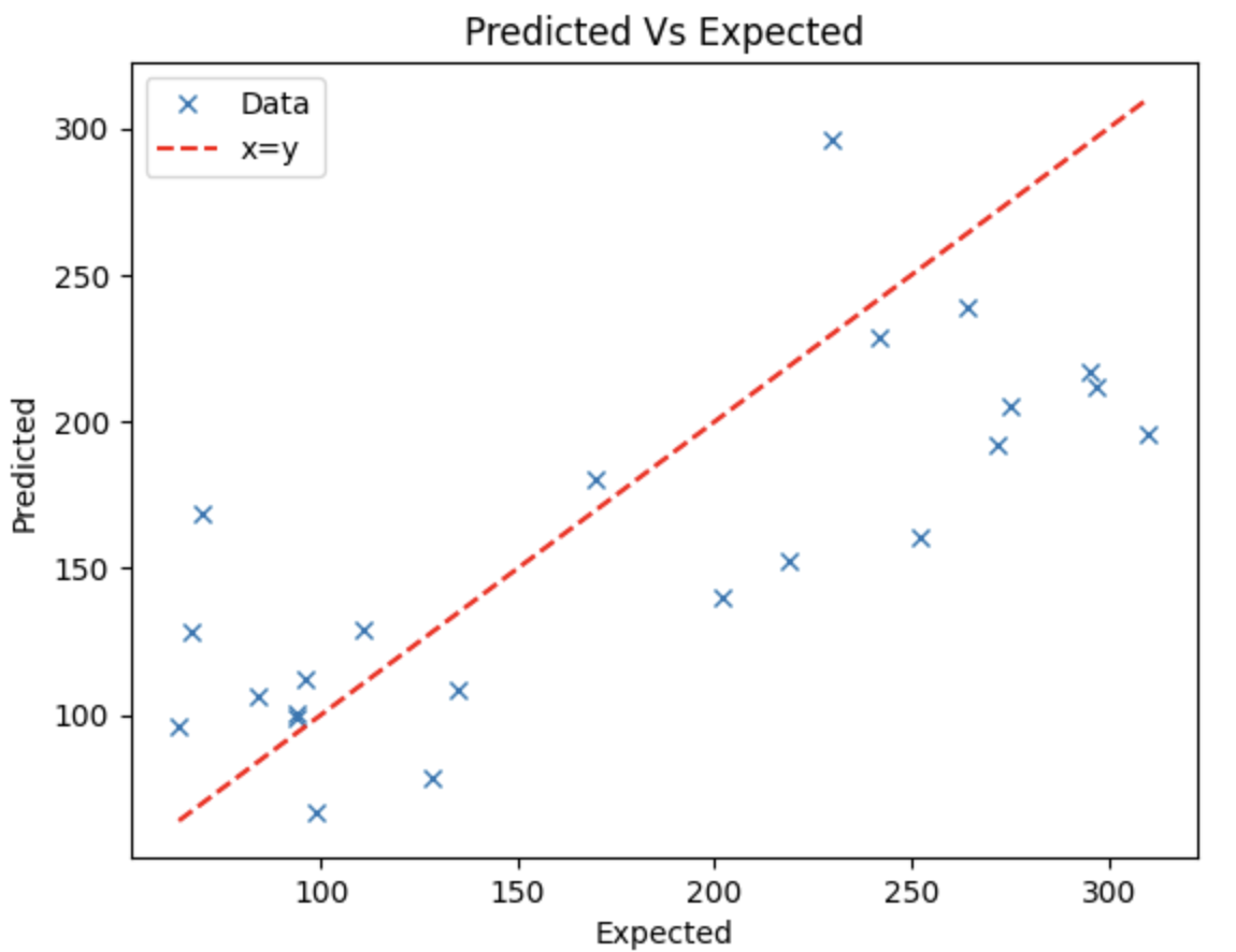

Of course, the predictions aren't perfect and likely never will be for most problems as all recorded data has some measurement error. Beyond measurement error, problems that we solve are typically not a result of simply physical processes. If they are a result of physical processes they are typically ones we don't fully understand (if we did then we wouldn't need a machine learning solution!). Given these two sources of uncertainty it is likely that you'll never have a model that can always produce perfect predictions, but you should still aim for it. The key is to balance the training time and cost against the accuracy gains you'll see. Aim for a model that produces predictions that satisfactory for your problem, trying to attain perfection can be expensive and time-consuming.

Summary

In this topic we've gone through a simple example of building a fully connected neural regression network. Next, have a look at the maths behind the neural network we've built in this topic:

Basics of Neural Networks