Least Squares Inversion

Defining a problem and a cost function

Let us assume that we have some data that we have acquired, $in d $in, and we want to understand the underlying physical parameters, $in m $in, that gave rise to this data through some mapping transformation that we will encode in what we will call a forward operator, $in G $in. Then the general form of our problem to solve is given by

$$d = Gm$$

Unless otherwise stated we'll assume that the data, $in d $in, and model, $in m $in, are from a Gaussian distribution and have associated errors, although we shall omit them for the time being and revisit them in the covariance matrices section. The choice of a Gaussian distribution is arbitrary but leads us to defining the following cost function (also referred to as a misfit function).

$$C = (d-Gm)^{T}(d-Gm)$$

As previously mentioned, we have omitted the data and model errors as well as any a priori model information. We'll leave this until the covariance section. For more mathematical rigour around these definitions please see the book "Inverse Theory Problems" by Albert Tarantola.

Solving over general problem

Starting with the general equation form of our problem statement we can now start to re-arrange this formula for the model variables, $in m $in, which we are interested in determining.

The first thing to note is that the forward operator, G, is typically a matrix with a size of $in N_{d} $in x $in N_{m} $in where $in N_{d} $in and $in N_{m} $in are the number of data samples and the number of model variables respectively. Although we will highlight this later, it might be obvious that this matrix can become very large and difficult to handle if either the number of data points or the dimensionality of the model space is large.

Given that $in G $in is a matrix then we can't simply divide both sides of the equation by G, unless it is a square matrix with non-zero determinant, in which case we can simply multiple both sides of the equation by the inverse of the forward operator to determine the solution, this is known as the Cramer solution. Therefore, generally, we must first "make G square". We can do this rather simply by multiplying on the left of this equation by the transpose of the forward operator matrix, $in G^{T} $in.

$$G^{T}d = G^{T}Gm$$

This means that the product $in G^{T}G $in now has dimensions of $in N_{s} $in x $in N_{s} $in, i.e. it is square. Now that we can be sure that this "squared" forward operator is square in dimensionality then we can multiple both sides of the equation by the inverse of this squared forward operator. Note that this would only make sense if $in G^{T}G $in is invertible, which is to say that it is over-determined in this case.

$$(G^{T}G)^{-1} G^{T}d = (G^{T}G)^{-1} (G^{T}G) m$$

As you would expect, a value multiplied by it's inverse is equal to one (with obvious exceptions for zero). So the $in (G^{T}G)^{-1}(G^{T}G) $in term on the right side of the equation disappears, leaving us with an equation to determine the model parameters, $in m $in, from the recorded data, $in d $in, and our understanding of the physical system, $in G $in. Putting the model vector on the left hand side of the equation now we have:

$$m = (G^{T}G)^{-1} G^{T}d$$

The advantage of assuming Gaussian probabilities, and using the least-squares method, is the relative ease of the solution, as we have seen. A disadvantage is that it is relatively sensitive to outlying data, a few data points with a large misfit can cause the optimization of a least squares problem to not converge.

Polynomial curve fitting example

Let's look a specific example of using this form of equation to solve a problem.

We'll try to fit a polynomial curve to a dataset, a typical and standard problem. The form of an n^th order polynomial is given by:

$$y = a_{n}x^{n} + a_{n-1}x^{n-1} + \ldots a_{2}x^{2} +a_{1}x + a_{0} $$

Here the collection of $in a $in coefficients define the model parameters that we are looking for as they determine the shape of the fitted curve. We also have the choice of what order of polynomial, $in n $in, to use to fit the data, which is denoted by the vector of values $in y $in.

$$G= \begin{bmatrix} x_{1}^{m} & x_{1}^{m-1} & \ldots & x_{1}^{2} & x_{1} & 1 \\ x_{2}^{m} & x_{2}^{m-1} & \ldots & x_{2}^{2} & x_{2} & 1 \\ \vdots & \vdots & \ddots & \vdots & \vdots & \vdots\\ x_{Nd}^{m} & x_{Nd}^{m-1} & \ldots & x_{Nd}^{2} & x_{Nd} & 1 \\ \end{bmatrix} $$

We are going to use a dataset of various characteristics of Olympic athletes. In this instance we are solely interested in the relationship between the height and weight of the athletes to determine if there is a relationship, what it might be, and to develop a model that can predict, based solely on height, what the weight of the athlete might be. This is just a toy example to showcase how to use the linear least squares framework we have outlined to fit these functions, in the introduction to data science series we'll look at how we can include more information from the dataset including some of the non-numeric data to make a more robust predictive model.

We will be using python to perform this analysis so first we'll import some libraries, read the data, and show the first few lines to see what the data looks like, which is always a good first step in any investigation.

import pandas as pd
import numpy as np
import matplotlib.pyplot as plt

df = pd.read_csv('athletes.csv')
print(df.head(5))
df_small = df.loc[:,['weight','height']].dropna()
height = df_small.height.values.T
weight = df_small.weight.values.T

Since fitting an n^th order polynomial is a rather generic task it makes sense to generate some functions such that we can re-run this kind of analysis with any other data in the future. Even though we are going to use a 2^nd order polynomial to fit out data, it is sensible to make a function that can fit any order of polynomial. We'll also write a function to help us plot the results as well.

def plotting(x, y, m, xlabel, ylabel, polynomial_degree):
    plt.figure()
    plt.plot(x,y,'x')
    plt.xlabel(xlabel)
    plt.ylabel(ylabel)
    plt.title(f'{ylabel} Vs {xlabel}')
    xfine = np.linspace(np.min(x), np.max(x), 10*len(x))
    G = makeG(xfine, polynomial_degree)
    yfine = np.dot(G,m)
    plt.plot(xfine,yfine,'r--')

def makeG(x, polynomial_degree):
    G = np.zeros((len(x), polynomial_degree + 1))
    for power in range(polynomial_degree+1):
        G[:,-1-power] = x**power
    return G

def linearInversion(x, y, polynomial_degree, lam):
    G = makeG(x, polynomial_degree)
    Gt = G.T
    GtG = np.dot(Gt, G)
    regularization = lam * np.eye(polynomial_degree + 1)
    GtGinv = np.linalg.inv(GtG + regularization)
    m = np.dot(np.dot(GtGinv, Gt), y)
    return m

def getCost(x, y, m, polynomial_degree):
    G = makeG(x, polynomial_degree)
    yhat = np.dot(G,m)
    cost = np.linalg.norm(y-yhat,2)
    return cost

Now that we have the data imported and all the functions we require to run our inversion, all that is left is to define the order of polynomial that we are going to use, 2 in this case, run the inversion, and view the results.

polynomial_degree = 2
model = linearInversion(weight, height, polynomial_degree, 0)
print(model)
print(getCost(weight, height, model, polynomial_degree))
plotting(weight, height, model, 'weight','height', polynomial_degree)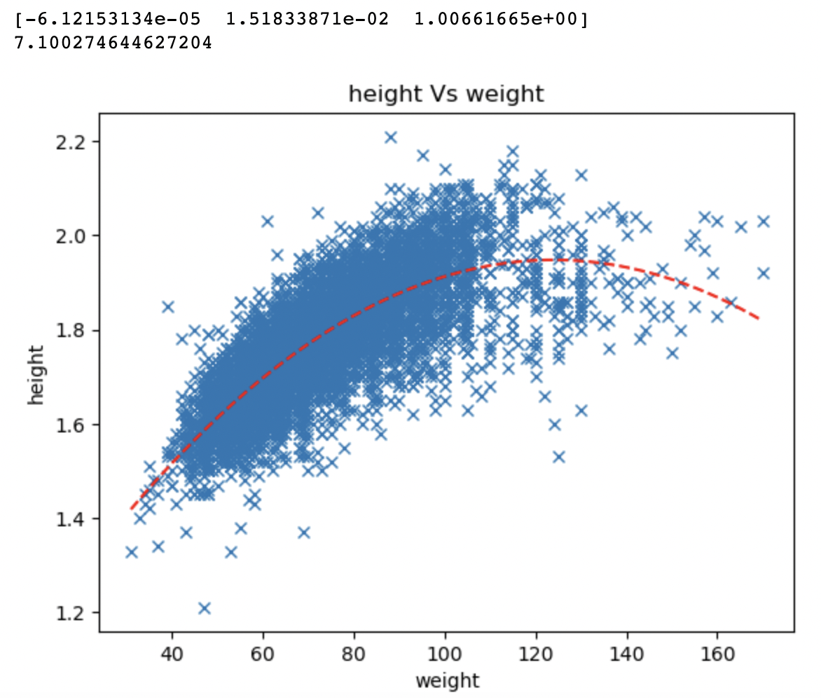

An alternative, and potentially more useful, derivation of the linear least squares equation

An alternative derivation of the Gauss-Newton method is formulate the problem as a cost function, which we have already done in the python python function "getCost", which defines the cost function as an L2-norm of the recorded data, $in d$in, and the estimated data based on the model parameters, $in \hat{d}$in. Where $in \hat{d} = G\hat{m} $in and $in \hat{m} $in is the current estimate of the model parameters.

$$C = ||d-Gm||^{2}$$

In this approach we want to minimize the cost function with regards to the model parameters. Which is to say, find me the model parameters which create estimated values as close to the recorded data as possible. We can do this by taking the first partial derivative of the cost function with respect to the model parameters and setting this to zero.

$$ \frac{\partial{C}}{\partial{m}} = \frac{\partial{||d-Gm||^{2}}}{\partial{m}} = 0$$

Even though this partial derivative involves matrices, the partial derivative is calculated in almost the same way as we would expected of single valued variables with one small exception.

Firstly, we can multiply out the brackets to remove the norm nomenclature from the equation

$$\frac{\partial{C}}{\partial{m}} = \frac{\partial{(d-Gm)^{T}(d-Gm)}}{\partial{m}} = 0$$ $$\frac{\partial{C}}{\partial{m}} = \frac{\partial{d^{T}d}}{\partial{m}} - \frac{m^{T}G^{T}d}{\partial{m}} - \frac{d^{T}Gm}{\partial{m}} + \frac{m^{T}G^{T}Gm}{\partial{m}} = 0$$

We can ignore the first terms as it is independent of $in m$in. We can also note that the partial derivative of $in m^{T}G^{T}d$in is the same as $in d^{T}Gm$in (they both equal $in d^{T}G$in) and in the final term can be solved in a similar way which leads us to the following equation

$$ -2d^{T}G + 2m^{T}GG^{T} = 0$$

We can then rearrange, divide by 2, and take the transpose of both sides of the equation to retrieve

$$ G^{T}d = mG^{T}G$$

An equation we have seen before and know how to re-arrange to retrieve the framework equation we derived above (see the start of this topic for detailed derivation).

We've shown how to perform linear least squares inversion (sometimes called Gauss-Newton inversion) and have gone through an example of using that framework to fit a polynomial curve to a dataset of athlete's weigh Vs height. But what about situations where the forward model isn't obviously linearly separable from the data? There are instances where this is the case, and we shall look at those in the introduction to non-linear inverse theory section. But first, let's look at an instance where the forward modeling operator doesn't look like it can be broken down into the constituent model and physics but can with a little mathematical trickery.

Simple mathematical tricks to force a linear problem